In-Class Exercise 2: Geospatial Data Wrangling

Published

January 16, 2023

Modified

March 6, 2023

Installing and loading sf, tidyverse, funModeling packages

pacman::p_load(sf, tidyverse,funModeling)

Handling Geospatial Data

Importing Geospatial Data

Importing geoBoundaries data set

geoNGA <- st_read("data/geospatial/",
                  layer = 
                  "geoBoundaries-NGA-ADM2") %>%
  st_transform(crs = 26392)

Reading layer `geoBoundaries-NGA-ADM2' from data source 
  `C:\gailteh\IS415-GAA\In-class_Ex\In-Class_Ex02\data\geospatial' 
  using driver `ESRI Shapefile'
Simple feature collection with 774 features and 6 fields
Geometry type: MULTIPOLYGON
Dimension:     XY
Bounding box:  xmin: 2.668534 ymin: 4.273007 xmax: 14.67882 ymax: 13.89442
Geodetic CRS:  WGS 84

Importing NGA data set

NGA <- st_read("data/geospatial/",
                  layer = 
                  "nga_admbnda_adm2_osgof_20190417") %>%
  st_transform(crs = 26392)

Reading layer `nga_admbnda_adm2_osgof_20190417' from data source 
  `C:\gailteh\IS415-GAA\In-class_Ex\In-Class_Ex02\data\geospatial' 
  using driver `ESRI Shapefile'
Simple feature collection with 774 features and 16 fields
Geometry type: MULTIPOLYGON
Dimension:     XY
Bounding box:  xmin: 2.668534 ymin: 4.273007 xmax: 14.67882 ymax: 13.89442
Geodetic CRS:  WGS 84

Importing Aspatial Data Set

Importing the water point data set and selecting only the water points within Nigeria

wp_nga <- read_csv("data/aspatial/WPdx.csv") %>%
  filter(`#clean_country_name` == "Nigeria")

Converting wkt data into sfc

wp_nga$Geometry = st_as_sfc(wp_nga$`New Georeferenced Column`)
wp_nga

# A tibble: 95,008 × 71
   row_id `#source`      #lat_…¹ #lon_…² #repo…³ #stat…⁴ #wate…⁵ #wate…⁶ #wate…⁷
    <dbl> <chr>            <dbl>   <dbl> <chr>   <chr>   <chr>   <chr>   <chr>  
 1 429068 GRID3             7.98    5.12 08/29/… Unknown <NA>    <NA>    Tapsta…
 2 222071 Federal Minis…    6.96    3.60 08/16/… Yes     Boreho… Well    Mechan…
 3 160612 WaterAid          6.49    7.93 12/04/… Yes     Boreho… Well    Hand P…
 4 160669 WaterAid          6.73    7.65 12/04/… Yes     Boreho… Well    <NA>   
 5 160642 WaterAid          6.78    7.66 12/04/… Yes     Boreho… Well    Hand P…
 6 160628 WaterAid          6.96    7.78 12/04/… Yes     Boreho… Well    Hand P…
 7 160632 WaterAid          7.02    7.84 12/04/… Yes     Boreho… Well    Hand P…
 8 642747 Living Water …    7.33    8.98 10/03/… Yes     Boreho… Well    Mechan…
 9 642456 Living Water …    7.17    9.11 10/03/… Yes     Boreho… Well    Hand P…
10 641347 Living Water …    7.20    9.22 03/28/… Yes     Boreho… Well    Hand P…
# … with 94,998 more rows, 62 more variables: `#water_tech_category` <chr>,
#   `#facility_type` <chr>, `#clean_country_name` <chr>, `#clean_adm1` <chr>,
#   `#clean_adm2` <chr>, `#clean_adm3` <chr>, `#clean_adm4` <chr>,
#   `#install_year` <dbl>, `#installer` <chr>, `#rehab_year` <lgl>,
#   `#rehabilitator` <lgl>, `#management_clean` <chr>, `#status_clean` <chr>,
#   `#pay` <chr>, `#fecal_coliform_presence` <chr>,
#   `#fecal_coliform_value` <dbl>, `#subjective_quality` <chr>, …

Converting wp_nga tibble data frame into sf data frame, then transforming into Nigeria PCS

wp_sf <- st_sf(wp_nga, crs=4326) %>%
  st_transform(crs = 26392)
wp_sf

Simple feature collection with 95008 features and 70 fields
Geometry type: POINT
Dimension:     XY
Bounding box:  xmin: 28907.91 ymin: 33736.93 xmax: 1293293 ymax: 1092883
Projected CRS: Minna / Nigeria Mid Belt
# A tibble: 95,008 × 71
   row_id `#source`      #lat_…¹ #lon_…² #repo…³ #stat…⁴ #wate…⁵ #wate…⁶ #wate…⁷
 *  <dbl> <chr>            <dbl>   <dbl> <chr>   <chr>   <chr>   <chr>   <chr>  
 1 429068 GRID3             7.98    5.12 08/29/… Unknown <NA>    <NA>    Tapsta…
 2 222071 Federal Minis…    6.96    3.60 08/16/… Yes     Boreho… Well    Mechan…
 3 160612 WaterAid          6.49    7.93 12/04/… Yes     Boreho… Well    Hand P…
 4 160669 WaterAid          6.73    7.65 12/04/… Yes     Boreho… Well    <NA>   
 5 160642 WaterAid          6.78    7.66 12/04/… Yes     Boreho… Well    Hand P…
 6 160628 WaterAid          6.96    7.78 12/04/… Yes     Boreho… Well    Hand P…
 7 160632 WaterAid          7.02    7.84 12/04/… Yes     Boreho… Well    Hand P…
 8 642747 Living Water …    7.33    8.98 10/03/… Yes     Boreho… Well    Mechan…
 9 642456 Living Water …    7.17    9.11 10/03/… Yes     Boreho… Well    Hand P…
10 641347 Living Water …    7.20    9.22 03/28/… Yes     Boreho… Well    Hand P…
# … with 94,998 more rows, 62 more variables: `#water_tech_category` <chr>,
#   `#facility_type` <chr>, `#clean_country_name` <chr>, `#clean_adm1` <chr>,
#   `#clean_adm2` <chr>, `#clean_adm3` <chr>, `#clean_adm4` <chr>,
#   `#install_year` <dbl>, `#installer` <chr>, `#rehab_year` <lgl>,
#   `#rehabilitator` <lgl>, `#management_clean` <chr>, `#status_clean` <chr>,
#   `#pay` <chr>, `#fecal_coliform_presence` <chr>,
#   `#fecal_coliform_value` <dbl>, `#subjective_quality` <chr>, …

Geospatial Data Cleaning

Excluding Redundant Fields

Retaining column 3,4,8 and 9

NGA <- NGA %>%
  select(c(3:4, 8:9))

Checking for duplicate name

Flag out LGA names that are duplicated

NGA$ADM2_EN[duplicated(NGA$ADM2_EN)== TRUE]

[1] "Bassa"    "Ifelodun" "Irepodun" "Nasarawa" "Obi"      "Surulere"

Correcting the errors of duplicate names

NGA$ADM2_EN[94] <- "Bassa, Kogi"
NGA$ADM2_EN[95] <- "Bassa, Plateau"
NGA$ADM2_EN[304] <- "Ifelodun, Kwara"
NGA$ADM2_EN[305] <- "Ifelodun, Osun"
NGA$ADM2_EN[355] <- "Irepodun, Kwara"
NGA$ADM2_EN[356] <- "Irepodun, Osun"
NGA$ADM2_EN[519] <- "Nasarawa, Kano"
NGA$ADM2_EN[520] <- "Nasarawa, Nasarawa"
NGA$ADM2_EN[546] <- "Obi, Benue"
NGA$ADM2_EN[547] <- "Obi, Nasarawa"
NGA$ADM2_EN[693] <- "Surulere, Lagos"
NGA$ADM2_EN[694] <- "Surulere, Oyo"

Checking that there are no more duplicate

NGA$ADM2_EN[duplicated(NGA$ADM2_EN)== TRUE]

character(0)

Data Wrangling for Water Point Data

Using freq() from funModeling package to show the distribution of water point status visually

freq(data = wp_sf,
     input = '#status_clean')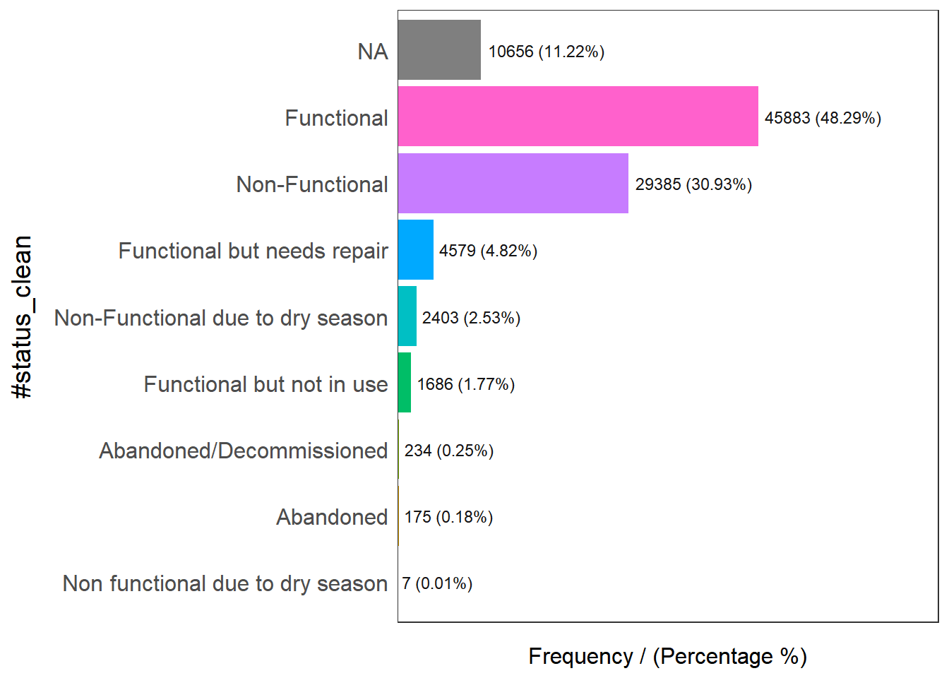

                     #status_clean frequency percentage cumulative_perc
1                       Functional     45883      48.29           48.29
2                   Non-Functional     29385      30.93           79.22
3                             <NA>     10656      11.22           90.44
4      Functional but needs repair      4579       4.82           95.26
5 Non-Functional due to dry season      2403       2.53           97.79
6        Functional but not in use      1686       1.77           99.56
7         Abandoned/Decommissioned       234       0.25           99.81
8                        Abandoned       175       0.18           99.99
9 Non functional due to dry season         7       0.01          100.00

rename() renames the column from #status_clean to status_clean, using select() to include status_clean in the output dataframe, mutate() and replace_na() are used to recode NA values into “unknown”

wp_sf_nga <- wp_sf %>%
  rename(status_clean = '#status_clean') %>%
  select(status_clean) %>%
  mutate(status_clean = replace_na(
  status_clean, "unknown"))

Extracting Water Point Data

Extracting functional water points

wp_functional <- wp_sf_nga %>%
  filter(status_clean %in%
           c("Functional",
             "Functional but not in use",
             "Functional but needs repair"))

Extracting non-functional water points

wp_nonfunctional <- wp_sf_nga %>%
  filter(status_clean %in%
           c("Abandoned/Decommissioned",
             "Abandoned",
             "Non-Functional due to dry season",
             "Non-Functional",
             "Non functional due to dry season"))

Extracting water points with unknown status

wp_unknown <- wp_sf_nga %>%
  filter(status_clean == "unknown")

Peforming EDA on the derived dataframes

freq(data = wp_functional,
     input = "status_clean")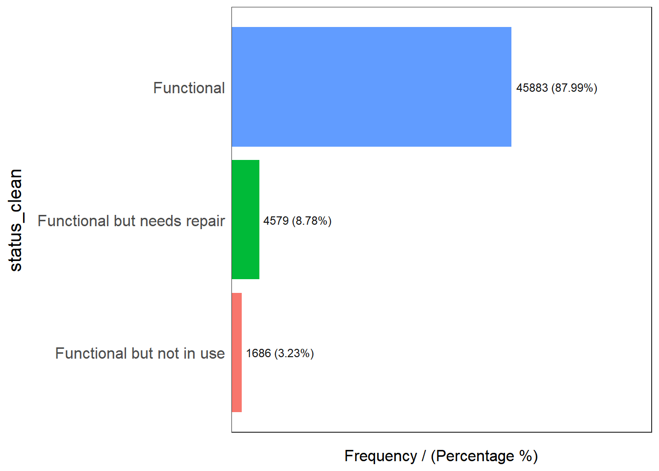

                 status_clean frequency percentage cumulative_perc
1                  Functional     45883      87.99           87.99
2 Functional but needs repair      4579       8.78           96.77
3   Functional but not in use      1686       3.23          100.00

freq(data = wp_nonfunctional,
     input = "status_clean")

                      status_clean frequency percentage cumulative_perc
1                   Non-Functional     29385      91.25           91.25
2 Non-Functional due to dry season      2403       7.46           98.71
3         Abandoned/Decommissioned       234       0.73           99.44
4                        Abandoned       175       0.54           99.98
5 Non functional due to dry season         7       0.02          100.00

freq(data = wp_unknown,
     input = 'status_clean')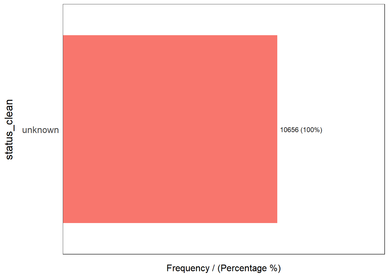

  status_clean frequency percentage cumulative_perc
1      unknown     10656        100             100

Point-in-polygon count

To find the number of total, functional, nonfunctional, and unknown water points in each LGA.

st_intersects() identifies all the water points for each type, then length() is used to calculate the number of water points for each type

NGA_wp <- NGA %>%
  mutate(`total_wp` = lengths(
    st_intersects(NGA, wp_sf_nga))) %>%
  mutate(`wp_functional` = lengths(
    st_intersects(NGA, wp_functional))) %>%
  mutate(`wp_nonfunctional` = lengths(
    st_intersects(NGA, wp_nonfunctional))) %>%
  mutate(`wp_unknown` = lengths(
    st_intersects(NGA, wp_unknown)))

Plotting distribution of total waterpoints in a histogram

ggplot(data = NGA_wp,
       aes(x = total_wp)) +
  geom_histogram(bins = 20,
                 color = "black",
                 fill = "light blue") +
  geom_vline(aes(xintercept=mean(
    total_wp, na.rm=T)),
              colour="red",
              linetype="dashed",
              size = 0.8) +
  ggtitle("Distribution of total water points by LGA") + 
  xlab("No. of water points") +
  ylab("No. of\nLGAs") +
  theme(axis.title.y= element_text(angle = 0))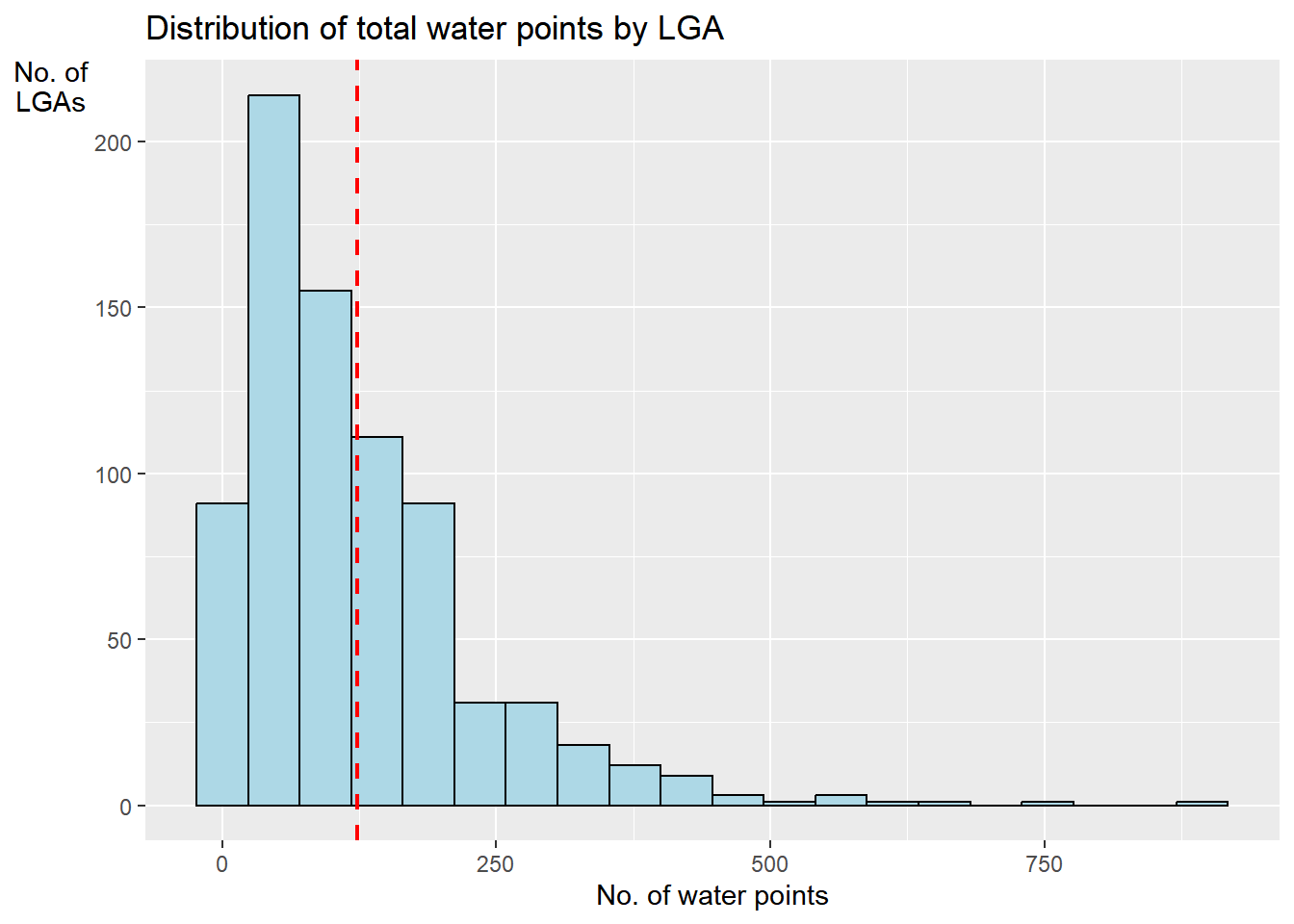

Exporting NGA_wp data frame into rds format

Retaining the sf object structure for subsequent analysis in the future.

write_rds(NGA_wp, "data/rds/NGA_wp.rds")