pacman::p_load(tmap, tidyverse, sf)In-Class Exercise 3: Analytical Mapping
1 Importing and loading packages
2 Importing Data
Importing NGA_wp.rds from In-Class Ex02
NGA_wp <- read_rds("data/rds/NGA_wp.rds")3 Plotting Choropleth Map
Saving maps into object p1 and p2, then plotting the maps
p1 <- tm_shape(NGA_wp) +
  tm_fill("wp_functional",
          n = 10,
          style = "equal",
          palette = "Blues") +
  tm_borders(lwd = 0.1,
             alpha = 1) +
  tm_layout(main.title = "Distribution of functional water point by LGAs",
            legend.outside = FALSE)
p2 <- tm_shape(NGA_wp) +
tm_fill("total_wp",
n = 10,
style = "equal",
palette = "Blues") +
tm_borders(lwd = 0.1,
alpha = 1) +
tm_layout(main.title = "Distribution of total water point by LGAs",
legend.outside = FALSE)tmap_arrange(p2, p1, nrow = 1)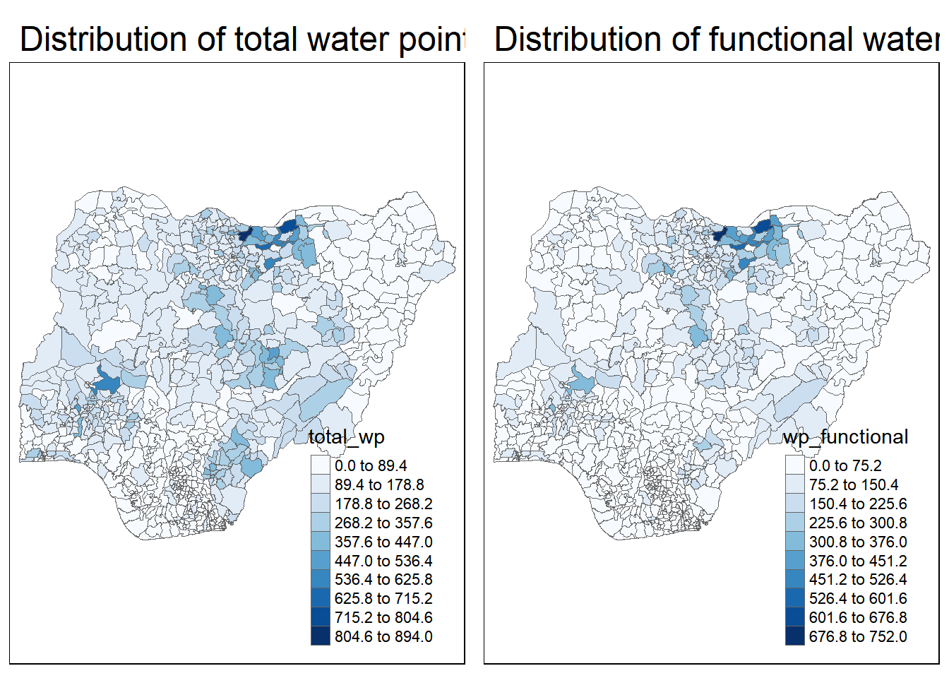
4 Choropleth Map for Rates
It is important to map rates rather than counts because water points are not equally distributed in space. If we do not account for how many water points are somewhere, we end up mapping total point size rather than the poic of interest
4.1 Deriving Proportion of Funtional & Non-Functional WP
Mutate() derives the fields pct_functional and pct_nonfunctional
NGA_wp <- NGA_wp %>%
  mutate(pct_functional = wp_functional/total_wp) %>%
  mutate(pct_nonfunctional = wp_nonfunctional/total_wp)
4.2 Plotting Map of rate
tm_shape(NGA_wp) +
  tm_fill("pct_functional",
          n = 10,
          style = "equal",
          palette = "Blues",
          legend.hist = TRUE) +
  tm_borders(lwd = 0.1,
             alpha = 1) +
  tm_layout(main.title = "Rate map of functional water point by LGA",
            legend.outside = TRUE)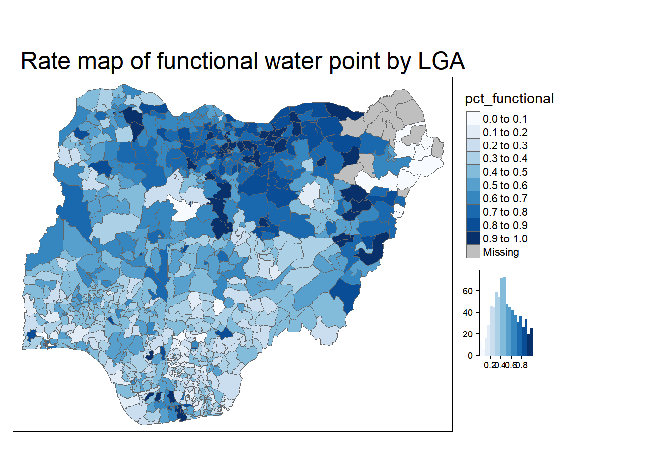
5 Extreme Value Maps
Variations of choropleth maps in which classification is designed to highlight extreme values at lower and upper ends of the scale (goal is to identify outliers).
5.1 Percentile Map
Quantile map with 6 specific categories (0-1%, 1-10%, 10-50%, 50-0%, 90-99%, 99-100%). Corresponding breakpoints are derived by means of the base R quantile command, passing an explicit vector of cumulative probabilities. Begin & end point needs to be included
5.1.1 Data Preparation
Excluding records with NA
NGA_wp <- NGA_wp %>%
  drop_na()
Creating customised classification and extracting values
percent <- c(0, .01, .1, .5, .9, .99, 1)
var <- NGA_wp["pct_functional"] %>%
  st_set_geometry(NULL)
quantile(var[,1], percent)
0% 1% 10% 50% 90% 99% 100%
0.0000000 0.0000000 0.2169811 0.4791667 0.8611111 1.0000000 1.0000000 When variables are extracted from an sf dataframe, the geometry is extracted as well. For mapping and spatial manipulations this is expected behavior, but many R functions cannot deal with geometry. quantile() will give an error. Hence, st_set_geometry(NULL) is used to drop the geometry field.
5.1.2 Creating Functions
Creating get.var function
This function extracts a variable (e.g. wp_nonfunctional) as a vactor out of an sf dataframe.
arguments: vname: variable name df: (name of the sf dataframe)
returns: v: a vector with values
get.var <- function(vname, df) {
  v <- df[vname] %>%
    st_set_geometry(NULL)
  v <- unname(v[,1])
  return(v)
}
Percentile Mapping Function
percentmap <- function(vnam, df, legtitle=NA, mtitle ="Percentile Map"){
  percent <- c(0, .01, .1, .5, .9, .99, 1)
  var <- get.var(vnam, df)
  bperc <- quantile(var, percent)
  tm_shape(df) +
  tm_polygons() +
  tm_shape(df) +
    tm_fill(vnam,
            title=legtitle,
            breaks=bperc,
            palette="Blues",
            labels=c("<1%", "1%-10%", "10%-50%", "50%-90%", "90%")) +
    tm_borders() +
    tm_layout(main.title = mtitle,
              title.position = c("right", "bottom"))
}
Running the function
percentmap("total_wp", NGA_wp)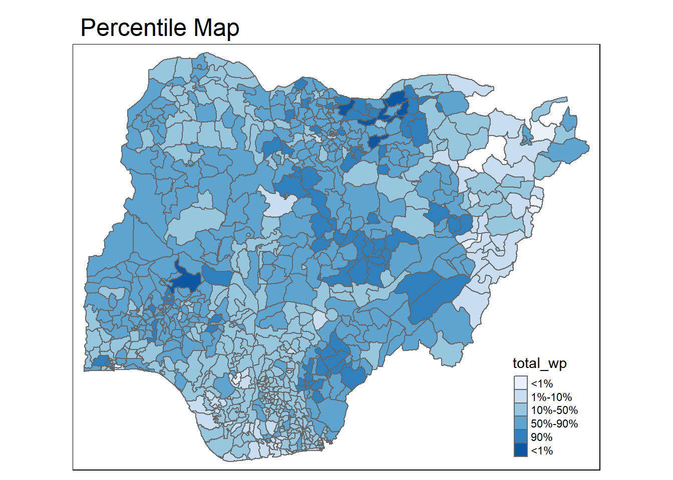
5.2 Box Map
An augmented quartile map with an additional lower and upper category. If there are lower outliers, starting point for the breaks is the minimum value, second break is the lower fence.
On the other hand, if there is no lower outliers, the starting point for the breaks is the lower fence, and the second break is the minimum value. There is no observations that fall in the interval between the lower fence and minimum value.
ggplot(data = NGA_wp,
       aes(x = "",
           y = wp_nonfunctional)) +
  geom_boxplot()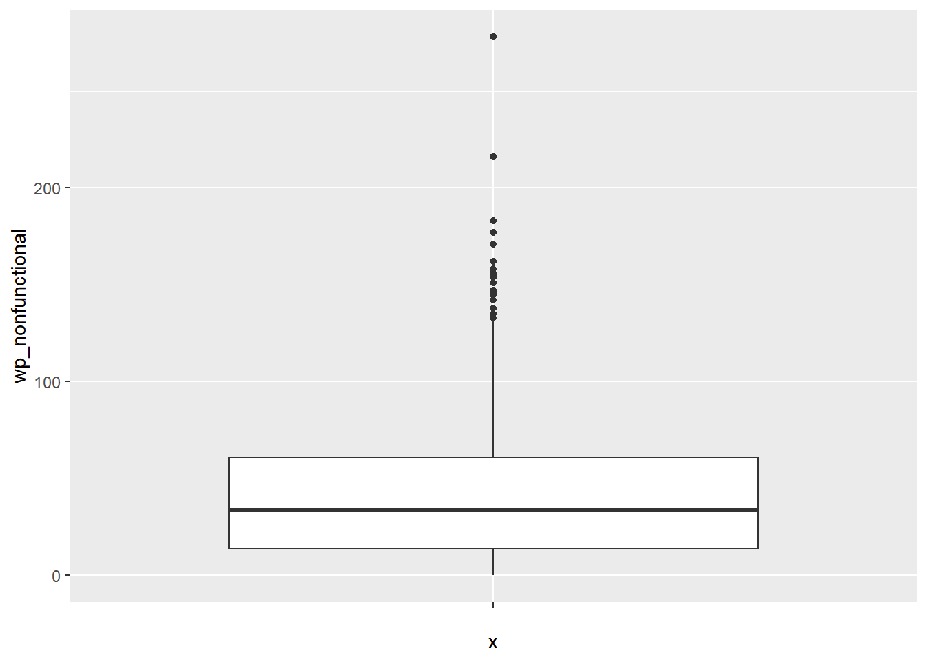
To create a box map, custom breaks specifications will be used. However, the break points will vary depending on whether there are lower/upper outliers.
5.2.1 Creatings functions
boxbreaks function
Creating break points for the box map.
It takes in the arguments v (a vector with multiple observations) and mult (multiplier for IQR, 1.5 by default). It returns bb, a vector with 7 break points compute quartile and fences
boxbreaks <- function(v, mult=1.5) {
  qv <- unname(quantile(v))
  iqr <- qv[4] - qv[2]
  upfence <- qv[4] + mult * iqr
  lofence <- qv[2] - mult * iqr

  # initialise break points vector
  bb <- vector(mode="numeric", length=7)

  # logic for lower and upper fence
  if (lofence < qv[1]) { # no lower outliers
    bb[1] <- lofence
    bb[2] <- floor(qv[1])
  } else {
    bb[2] <- lofence
    bb[1] <- qv[1]
  }

  if (upfence > qv[5]) { # no upper outliers
    bb[7] <- upfence
    bb[6] <- ceiling(qv[5])
  } else {
    bb[6] <- upfence
    bb[7] <- qv[5]
  }

  bb[3:5] <- qv[2:4]
  return(bb)
}
get.var function
get.var <- function(vname,df) {
  v <- df[vname] %>% st_set_geometry(NULL)
  v <- unname(v[,1])
  return(v)
}
Testing the function
var <- get.var("wp_nonfunctional", NGA_wp)
boxbreaks(var)
[1] -56.5 0.0 14.0 34.0 61.0 131.5 278.0Boxmap function
Function to create box map.
boxmap <- function(vnam, df,
                   legtitle=NA,
                   mtitle = "Box Map",
                   mult = 1.5) {
  var <- get.var(vnam, df)
  bb <- boxbreaks(var)
  tm_shape(df) +
    tm_polygons() +
  tm_shape(df) +
    tm_fill(vnam, title=legtitle,
            breaks=bb,
            palette="Blues",
            labels = c("lower outlier",
                       "< 25%",
                       "25% - 50%",
                       "50% - 75%",
                       ">75%",
                       "upper outlier")) +
    tm_borders() +
    tm_layout(main.title = mtitle,
              title.position = c("left", "top"))
}tmap_mode("plot")
boxmap("wp_nonfunctional", NGA_wp)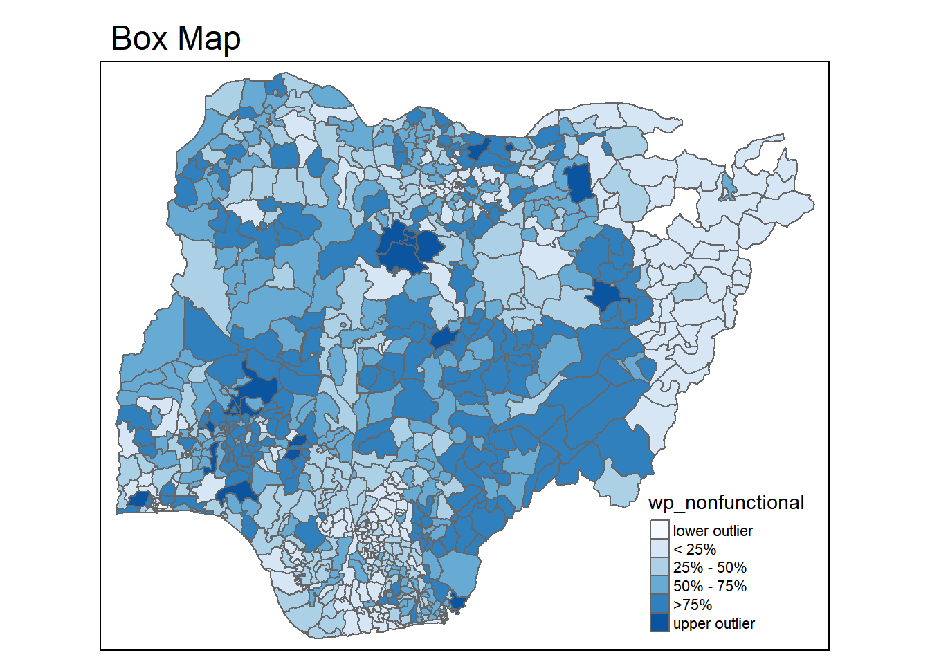
NGA_wp <- NGA_wp %>%
  mutate(wp_functional = na_if(
    total_wp, total_wp < 0))